Tuning Guide#
Partitions and Parallelism#
The goal of any distributed compute engine is to parallelize work as much as possible, allowing the work to scale by adding more compute resource.
The basic unit of concurrency and parallelism in Ballista is the concept of a partition. The leaf nodes of a query
are typically table scans that read files from object storage, and the number of partitions such a scan produces is
driven by datafusion.execution.target_partitions. This is currently a global setting for the entire context.
DataFusion’s own default for this setting is the number of CPU cores available to the process. Ballista overrides it
to 16 in SessionConfig::new_with_ballista(), so a context created with SessionContext::remote() or
SessionContext::standalone() starts at 16. If you instead build your own SessionConfig and pass it to
remote_with_state() or standalone_with_state(), Ballista leaves the setting alone and you get whatever that
config carries, which is the client machine’s core count for a plain SessionConfig::new(). Set it explicitly if
you care about the value.
A scan is partitioned in two steps:
When the table is listed, its files are sorted by path and distributed into at most
target_partitionsfile groups. A “customer” table of 200 Parquet files read withtarget_partitions = 16therefore produces 16 partitions of roughly 13 files each, not 200 partitions.The physical optimizer then splits individual files by byte range, so a table with fewer files than
target_partitionscan still be read in parallel. A table consisting of a single large Parquet file is split intotarget_partitionsbyte ranges rather than being read by one task. This step is controlled bydatafusion.optimizer.repartition_file_scans(defaulttrue) and only applies when the scan reads at leastdatafusion.optimizer.repartition_file_min_sizebytes (default 10 MB). Small tables below that threshold are left as a single partition, since splitting them costs more than it saves.
Ballista disables DataFusion’s round-robin repartitioning, so this file-group splitting is the only source of
parallelism for a scan stage. Raising target_partitions is the way to increase it, and lowering it is the way to
reduce the number of partitions a large table is read with.
Example: Setting the desired number of shuffle partitions when creating a context.
use ballista::extension::{SessionConfigExt, SessionContextExt};

let session_config = SessionConfig::new_with_ballista()
    .with_target_partitions(200);

let state = SessionStateBuilder::new()
    .with_default_features()
    .with_config(session_config)
    .build();

let ctx: SessionContext = SessionContext::remote_with_state(&url,state).await?;
Partitions and Tasks#
A stage’s partition count is not the same as its task count. The scheduler keeps a cursor over the stage’s
partitions and, each time an executor is assigned work, hands out a slice of those partitions to run as a single
task. The size of that slice is bounded by both the executor’s free vcores and
ballista.scheduler.max_partitions_per_task.
That setting defaults to 0, meaning the cap is removed and each task is filled up to the assigned executor’s free
vcore count: a 16-partition stage runs as one task on an idle 16-vcore executor, or as four 4-partition tasks
across four 4-vcore executors. This reduces task count and scheduling overhead and allows operators such as sort
and hash join to work across partitions within a task.
Set it to 1 to get one task per partition, or to any positive value to cap the slice size.
key |
type |
default |
description |
|---|---|---|---|
ballista.scheduler.max_partitions_per_task |
UInt64 |
0 |
Upper bound on the number of input partitions packed into a single task’s |
Stages whose plan collapses all input into a single partition (for example under a CoalescePartitionsExec or
SortPreservingMergeExec) ignore this cap and always pack their full pending queue into one task, since splitting
them would produce partial results that downstream stages cannot merge.
Each task’s plan is rewritten before dispatch so that its scan sees only the file groups belonging to its own slice.
Configuring Executor vcores#
Each executor instance advertises a fixed number of virtual cores (vcores) to the scheduler. This is specified by
passing a --vcores command-line parameter. The default setting is to use all available CPU cores.
Increasing this configuration setting will increase the number of tasks that each executor can run concurrently but this will also mean that the executor will use more memory. If executors are failing due to out-of-memory errors then decreasing the vcore count may help.
Configuring Executor Memory Pool#
By default the executor auto-sizes a bounded memory pool from the detected
host or cgroup memory limit, so spillable operators (sort, hash join, hash
aggregate) spill to disk under pressure instead of growing until the host
runs out of memory. The pool is sized to --memory-pool-fraction (default
0.70, i.e. 70%) of the detected limit, so headroom is left for untracked
overhead such as in-flight Arrow batches, shuffle writer buffers, and
fragmentation. When running under a cgroup-limited container (the common
Kubernetes/Docker case), the cgroup limit is used in preference to host
memory when it is the tighter of the two.
To use a specific budget instead of auto-detection, pass --memory-pool-size
when starting the executor:
ballista-executor --memory-pool-size 8GB --vcores 8
The argument accepts human-readable sizes (8GB, 512MiB) or a plain byte
count. SI suffixes (KB/MB/GB) are powers of 10; IEC suffixes
(KiB/MiB/GiB) are powers of 2. Pass --memory-pool-size 0 to opt out of
the pool entirely and run DataFusion’s unbounded pool, matching the executor’s
pre-auto-sizing behavior.
Whether the budget comes from auto-detection or --memory-pool-size, it is
divided equally across the executor’s vcores: each task receives its own
FairSpillPool of size memory_pool_size / vcores. With
--memory-pool-size 8GB --vcores 8, every task sees a 1 GB pool, fully
isolated from other tasks. Idle slots do not lend their share to busy ones,
which keeps task memory predictable at the cost of some unused capacity when
the executor is under-utilized.
Choosing the Executor’s Memory Allocator#
The ballista-executor binary uses mimalloc
as its global allocator by default. To use
jemalloc instead, build it with the
jemalloc feature, which takes precedence over mimalloc:
cargo install --locked ballista-executor --features jemalloc
Allocators differ in how much memory they hold on to after it is freed, so the choice can change an executor’s resident memory as well as its speed. The memory pool described above counts reservations, not resident memory, so leave headroom whichever allocator you use. jemalloc is not supported on Windows (MSVC) targets.
The executor refuses to start if the per-task share would round to zero (i.e.
memory_pool_size < vcores).
Use --memory-pool-fraction to tune how much of the detected memory limit
the auto-sized pool uses; it accepts a value in (0.0, 1.0] and defaults to
0.70. It is ignored when --memory-pool-size is set.
Because operators spill to disk rather than fail, make sure the executor’s
--work-dir has enough scratch space to absorb spills under memory pressure.
DataFusion caps spill files at 100 GB per runtime by default, and a query that
spills more fails with “The used disk space during the spilling process has
exceeded the allowable limit”. Large sorts and sort-merge joins can exceed this
at high scale factors. Raise the cap with --max-temp-directory-size, which
takes the same size values as --memory-pool-size:
ballista-executor --memory-pool-size 48GB --max-temp-directory-size 1TB
The limit applies to each session’s runtime on the executor, shared by that
session’s tasks. Setting datafusion.runtime.max_temp_directory_size on the
client has no effect on executors.
Join Strategy#
How Ballista picks a join depends on whether adaptive query execution is on.
With AQE (the default)#
AQE chooses each join at runtime, from measured sizes, after the join’s inputs
have run. It turns both hash joins and sort-merge joins into a single runtime
node and decides from that evidence, so datafusion.optimizer.prefer_hash_join
has no effect here.
Broadcast. If the smaller side is under
ballista.optimizer.broadcast_join_threshold_bytes(128 MiB by default) and the join type allows it, that side is broadcast and the join runs as aCollectLefthash join, without shuffling the larger side.Partitioned hash join. Otherwise both sides are shuffled on the join key, and the join runs as a hash join when every build partition is under
ballista.optimizer.hash_join_max_build_partition_bytes(64 MiB by default).Sort-merge join. A build partition over that limit falls back to sort-merge join, which spills to disk under memory pressure.
When a build side’s size is only an estimate, AQE can shuffle that side on its own first to measure it, so a join whose build side was over-estimated can still be broadcast. See What AQE does today.
Setting ballista.optimizer.hash_join_max_build_partition_bytes to 0 disables
the per-partition check, so AQE uses a hash join regardless of build size and
sort-merge join becomes unreachable.
With AQE turned off#
The static planner keeps DataFusion’s physical planning choice.
SessionConfig::new_with_ballista() sets datafusion.optimizer.prefer_hash_join
to false, so joins are planned as sort-merge joins by default. This is the
opposite of DataFusion’s standalone default and reflects two facts:
DataFusion’s hash join implementation does not yet support spilling: the full build side must fit in memory per task.
Ballista executors run multiple tasks in parallel per host, so per-task build sides aggregate quickly under load and can OOM the executor.
Sort-merge join spills under memory pressure via the executor’s memory pool, making it the safer default for distributed execution.
The static planner only promotes hash joins to broadcast, so with this default Ballista does not broadcast joins. If you know the build side of a particular query fits comfortably in memory and you want hash-join performance, including broadcast promotion, opt back in at the session level:
SET ballista.planner.adaptive.enabled = false;
SET datafusion.optimizer.prefer_hash_join = true;
or in code:
let session_config = SessionConfig::new_with_ballista()
    .set_bool("ballista.planner.adaptive.enabled", false)
    .set_bool("datafusion.optimizer.prefer_hash_join", true);
These settings apply per session and do not require restarting the scheduler or executors.
Shuffle Implementation#
Ballista exchanges data between query stages by writing the output of each upstream task to local files, which downstream tasks read either from disk (when co-located) or over Arrow Flight. Ballista uses a sort-based shuffle writer that bounds file count and memory use. Single-partition stages (a query’s final output, coalesce, and broadcast-build stages) are written directly to one file.
Sort-based shuffle#
The sort-based writer accumulates incoming batches in memory, tracking each row’s output partition. It spills the buffered batches to disk when either of two independent triggers fires:
the runtime memory pool rejects a growth request (the executor is under memory pressure — see Configuring Executor Memory Pool), or
the per-task buffered-bytes budget (
ballista.shuffle.sort_based.memory_limit_per_task_bytes) is reached. This budget is counted independently of the memory pool, so it bounds the writer’s memory even when the pool is unbounded (--memory-pool-size 0). Setting it to0disables this trigger, leaving memory-pool pressure as the sole spill signal.
Warning: setting memory_limit_per_task_bytes to 0 while the executor
runs an unbounded memory pool (--memory-pool-size 0) disables both spill
triggers. The writer then buffers the entire task’s shuffle output in memory
and never spills, which can exhaust the executor and cause an out-of-memory
failure on large inputs. Only use 0 together with a bounded memory pool (the
default; see
Configuring Executor Memory Pool), so
pool pressure still forces spilling.
At the end of input, the writer encodes each output partition’s buffered rows
and reserves the encoded bytes from the memory pool. A partition whose bytes
the pool refuses is appended to its spill file instead. The per-task budget
does not apply to this step, so only memory-pool pressure can make it spill.
With an unbounded pool (--memory-pool-size 0) it never does.
The task’s in-memory data and any spilled batches are then written into a single consolidated Arrow IPC file per task, alongside an index file that lets readers seek directly to a given output partition.
This produces two files per task instead of one per input and output partition pair, coalesces small batches to a target size before writing, and bounds shuffle memory use via spilling.
Worst-case sort-shuffle memory per executor is approximately
vcores × memory_limit_per_task_bytes, since one writer task can run per
core. Lower the per-task budget on memory-constrained executors to spill
sooner, or raise it to keep more data in memory and reduce spill I/O. Setting it
to 0 removes the budget entirely and is safe only with a bounded memory pool
(see the warning above).
The following session-level keys tune its behavior:
key |
type |
default |
description |
|---|---|---|---|
ballista.shuffle.sort_based.batch_size |
UInt64 |
8192 |
Target batch size in rows for coalescing small batches in sort shuffle |
ballista.shuffle.sort_based.memory_limit_per_task_bytes |
UInt64 |
268435456 |
Per-task buffered-bytes budget at which the sort shuffle writer spills its in-memory batches to disk. Counted independently of the runtime memory pool, so spilling kicks in even when the pool is unbounded. Total worst-case sort shuffle memory per executor is approximately vcores * this value. Set to 0 to disable the per-task budget and rely solely on runtime memory-pool pressure to trigger spilling; this is safe only with a bounded memory pool, otherwise the writer never spills and may run out of memory. |
Partition-id shuffles#
A hash shuffle assigns rows to partitions with DataFusion’s hash. That is consistent within a job, so joins and aggregations over shuffled inputs are correct, but it can’t match data already partitioned by another function. Spark partitions by Murmur3, for example, and a Spark-bucketed table read without a shuffle only lines up with a shuffled input if the shuffle places rows the same way.
A client that submits its own physical plan can do the placement itself. Put a
PartitionIdRepartitionExec where a hash RepartitionExec would go, and have
the plan below it compute each row’s output partition into an integer column:
use ballista_core::execution_plans::PartitionIdRepartitionExec;

// `plan` produces (key, value, pid): the id is column 2, and there are 8
// output partitions.
let shuffle = PartitionIdRepartitionExec::try_new(plan, 2, 8)?;
Output partition i holds exactly the rows whose id is i. The id column is
dropped before the rows are written, so whatever reads the shuffle sees the
input’s columns without it (the id can’t be the input’s only column). A null,
negative or out-of-range id fails the task.
Some things to keep in mind:
The node only marks the boundary and can’t be executed. The static planner replaces it with a stage that ends in the sort-based writer. The adaptive planner rejects it, because it may coalesce or re-plan an exchange’s partitions, which would break the placement. Set
ballista.planner.adaptive.enabledtofalseif a plan containing the node would otherwise be planned adaptively. Pipelined execution only shuffles by hash, so it rejects the node too.The shuffle’s output is reported as unknown partitioning, whatever function produced the ids, so operators that require hash-partitioned input won’t see their requirement met. Put the node under operators that declare no distribution requirement, such as a fragment node that does its joins and aggregations internally.
BallistaPhysicalExtensionCodecserializes the node, so a plan that contains it can be submitted over gRPC. A custom physical codec only needs to delegate to it, as in the extensions example.
Adaptive Query Execution#
Ballista runs adaptive query execution (AQE) by default: the scheduler re-runs the DataFusion physical optimizer between query stages. This lets the planner make decisions using statistics collected from completed stages rather than relying solely on pre-execution estimates.
To fall back to the static distributed planner, set
ballista.planner.adaptive.enabled to false on your SessionConfig:
let session_config = SessionConfig::new_with_ballista()
    .set_bool("ballista.planner.adaptive.enabled", false);
Configuration#
key |
type |
default |
description |
|---|---|---|---|
ballista.optimizer.broadcast_join_threshold_bytes |
UInt64 |
134217728 |
Byte-size threshold below which a hash join’s smaller side is promoted to CollectLeft and lowered via the broadcast pattern. Governs broadcast selection under both the static distributed planner and adaptive query planning (AQE). It also caps null-aware anti joins with a known build size because they require single-task CollectLeft execution. Set to 0 to disable promotion and reject null-aware anti joins. |
ballista.optimizer.broadcast_join_threshold_rows |
UInt64 |
1000000 |
Row-count threshold below which a hash join’s smaller side is promoted to CollectLeft and lowered via the broadcast pattern, used as a fallback when byte-size statistics are unavailable. Applies to adaptive query planning (AQE). Set to 0 to disable promotion via the row-count path. |
ballista.planner.adaptive.enabled |
Boolean |
true |
Enables Adaptive Query Planning: joins and partition counts are chosen from measured runtime statistics instead of planning-time estimates. Set to false to use the static distributed planner. |
What AQE does today#
When AQE is enabled, the scheduler builds the stage DAG incrementally. As each shuffle stage completes, the planner re-optimizes the remaining plan and emits the next set of runnable stages. The following adaptive optimizations are currently implemented:
Join selection. Each join is resolved from the runtime statistics of its completed input stages. The smaller side, compared by byte size and falling back to row count when sizes are unavailable, becomes the build side. When it falls under
ballista.optimizer.broadcast_join_threshold_bytes(or the row-count fallback), it is broadcast (CollectLeft) instead of shuffled. Null-aware anti joins useCollectLeftwith a single probe task because their state cannot be coordinated across executors. A known oversized build side is rejected instead of producing an incorrect distributed result. In practice mostNOT IN (subquery)predicates never plan a null-aware join at all:ballista.optimizer.not_in_subquery_rewrite(enabled by default) rewrites them into a fully distributable anti join plus a one-row count aggregate during logical optimization.Build-side staging. When a join’s build side has only an estimated size, the join type can be broadcast, the probe side is at least
ballista.optimizer.stage_build_side_min_probe_ratiotimes larger (10 by default), and the estimate is no more thanballista.optimizer.stage_build_side_max_estimate_multipletimes the broadcast threshold (32 by default), AQE shuffles the build side on its own first and reads back its measured size before choosing the join. A side that turns out small enough is broadcast, so the much larger probe side is never shuffled. Enabled by default; setballista.optimizer.stage_build_sidetofalseto shuffle both sides at once.Empty stage elimination. When a completed stage produces zero rows, its downstream exchange is replaced with an empty execution node, and emptiness is propagated up the plan so downstream stages are skipped entirely.
Shuffle-partition coalescing. Adjacent small output partitions of a completed stage are merged so the next stage runs fewer, larger tasks, down to a single task when the whole shuffle fits in
ballista.planner.coalesce.target_partition_bytes. Disabled by default; enable withballista.planner.coalesce.enabledand tune with theballista.planner.coalesce.*keys documented in Configuration.Parallel windows. Bounded
RANGE-frame windows are rewritten into a distributed range shuffle soBoundedWindowAggExecis not a serial bottleneck. Disabled by default; enable withballista.planner.parallel_window.enabled.Exchange reuse. When a query reads the same subplan more than once, such as a common table expression joined to itself or TPC-H q15’s revenue view, the subplan’s shuffle stage runs once and every reader reads its output. Subplans with a volatile expression such as
random(), and range-shuffled subplans, are never shared. Enabled by default; setballista.planner.reuse_exchange.enabledtofalseto run each copy.
Current limitations#
The implementation covers the happy path only. The following are known to be missing or incomplete:
Executor failure handling on the AQE path (#1986): a job that loses the output of a stage that has already finished fails instead of rerunning the stage
Switching from hash join to sort-merge join based on runtime statistics (#1988)
Switching from streaming aggregation to hash aggregation based on runtime statistics (#1989)
Set ballista.planner.adaptive.enabled to false to fall back to the static
distributed planner if you hit one of these. See
issue #1359 for the
tracking epic and ongoing work.
Caching DataFrames#
DataFrame::cache() does nothing by default (ballista.cache.noop = true).
With it turned off, the first action on a cached DataFrame runs the cached part
as a job of its own and keeps its output on the executors; later actions in the
same session read that output instead of recomputing it.
ctx.sql("SET ballista.cache.noop = false").await?;
let cached = ctx.table("t").await?.filter(col("x").gt(lit(5)))?.cache().await?;
cached.clone().count().await?; // builds the cache, then reads it
cached.collect().await?;       // reads it
Cached data is shuffle output on the executors. If a query loses part of it (an executor holding it is lost, or a fetch from it fails), it rebuilds the cache and carries on. A query planned by the adaptive planner, a pipelined query once its tasks have started, or one that also reads the lost cache, or a cache it was built from, another way (a self-join of a cached frame, say), fails instead with “lost DataFrame::cache() data; retry the query”, and the retry rebuilds the cache.
Cached data is not evicted yet: it is kept until it is found lost, or its session is removed through the scheduler’s
RemoveSessiongRPC call, which the Rust and Python clients do not expose yet. So cache only what you reuse. Eachcache()call caches its DataFrame anew; an earlier call’s cache is not freed.EXPLAINof a cached DataFrame never builds it.An operator can turn caching off for the whole cluster with the scheduler’s
--disable-dataframe-cacheflag; cached DataFrames are then computed as part of each query.
A cache works in both execution modes. Its build always runs staged, and queries over it run in the session’s mode, so a pipelined session reads a cache with streaming queries.
A full example, in staged and pipelined modes, from
examples/examples/standalone-dataframe-cache.rs:
//! `DataFrame::cache()` keeps a DataFrame's result on the executors, so queries
//! over it read the stored result instead of computing it again.
//!
//! This example:
//! 1. turns caching on (it is off by default),
//! 2. caches a prepared DataFrame (nothing runs yet),
//! 3. builds the cache with the first query and reads it with the next ones,
//!    in staged mode,
//! 4. switches the session to pipelined mode, which reads the same cache,
//! 5. runs three pipelined queries in parallel, printing rows as they arrive.
//!
//! Good to know: a cache belongs to its session and is not evicted yet, so
//! cache only what you reuse. Cached data lost with an executor is rebuilt, and
//! `EXPLAIN` never builds a cache. See the tuning guide for details.

use ballista::datafusion::{
    arrow::{record_batch::RecordBatch, util::pretty::pretty_format_batches},
    common::Result,
    execution::{SessionStateBuilder, options::CsvReadOptions},
    functions_aggregate::expr_fn::{count, sum},
    prelude::{DataFrame, SessionConfig, SessionContext, col, lit},
};
use ballista::prelude::{SessionConfigExt, SessionContextExt};
use ballista_examples::test_util;
use futures::StreamExt;

#[tokio::main]
async fn main() -> Result<()> {
    // 1. A standalone cluster, with caching turned on. Queries start staged.
    let ctx = standalone().await?;

    // 2. The DataFrame the queries start from. Nothing runs here: `cache()`
    //    only marks it to be kept. In an application this is the expensive
    //    part, such as scans, joins and aggregations.
    let path = format!("{}/aggregate_test_100.csv", test_util::examples_test_data());
    let sales = ctx
        .read_csv(path, CsvReadOptions::new())
        .await?
        .select(vec![
            col("c1").alias("category"),
            col("c2").alias("store"),
            col("c4").alias("amount"),
        ])?
        .filter(col("amount").gt(lit(0)))?
        .cache()
        .await?;

    // 3. Staged: the first query builds the cache, as a staged job, and then
    //    reads it. Later queries, and DataFrames derived from `sales`, read it.
    println!("== staged: the first query builds the cache ==");
    println!("{} sales", sales.clone().count().await?);

    println!("== staged: later queries read the cache ==");
    let staged = by_category(sales.clone())?.collect().await?;
    println!("{}", pretty_format_batches(&staged)?);

    // 4. Pipelined: one SET. A DataFrame keeps the settings of the session it
    //    came from, so rebuild it from the session's state to pick up the new
    //    mode. The plan, and the cache it reads, are the same.
    ctx.sql("SET ballista.execution.mode = 'pipelined'").await?;
    let sales = DataFrame::new(ctx.state(), sales.into_unoptimized_plan());

    // 5. Three queries in parallel, each streaming its rows from the cache as
    //    they are produced. Read every stream you start, and keep the queries
    //    running at once within the cluster: each holds the vcores of its
    //    widest stage until it ends, here 8 vcores / 2 partitions = 4 at once.
    println!("== pipelined: three queries in parallel ==");
    let (pipelined, _, _) = tokio::try_join!(
        stream("by category", by_category(sales.clone())?),
        stream(
            "sales per store",
            sales
                .clone()
                .aggregate(vec![col("store")], vec![count(lit(1)).alias("sales")])?
        ),
        stream(
            "top 5 amounts",
            sales
                .clone()
                .sort(vec![col("amount").sort(false, false)])?
                .limit(0, Some(5))?
        ),
    )?;

    // The cache gives the same result in either mode.
    assert_eq!(
        pretty_format_batches(&staged)?.to_string(),
        pretty_format_batches(&pipelined)?.to_string(),
    );
    Ok(())
}

/// Total amount per category, a query over the cached `sales`.
fn by_category(sales: DataFrame) -> Result<DataFrame> {
    sales
        .aggregate(
            vec![col("category")],
            vec![sum(col("amount")).alias("total")],
        )?
        .sort_by(vec![col("category")])
}

/// Starts a standalone cluster that can run staged and pipelined queries, and
/// returns a session on it with caching turned on.
async fn standalone() -> Result<SessionContext> {
    let mut config = SessionConfig::new_with_ballista()
        .with_target_partitions(2)
        .with_ballista_standalone_parallelism(8);
    // Pipelined queries need the scheduler to push tasks to executors.
    config
        .options_mut()
        .set("ballista.standalone.task_scheduling_policy", "push-staged")?;
    // `DataFrame::cache()` does nothing unless caching is turned on.
    config.options_mut().set("ballista.cache.noop", "false")?;

    let state = SessionStateBuilder::new()
        .with_config(config)
        .with_default_features()
        .build();
    SessionContext::standalone_with_state(state).await
}

/// Runs `df`, printing each batch of rows as it arrives, and returns them.
async fn stream(name: &str, df: DataFrame) -> Result<Vec<RecordBatch>> {
    let mut stream = df.execute_stream().await?;
    let mut batches = vec![];
    while let Some(batch) = stream.next().await {
        let batch = batch?;
        println!(
            "{name}:\n{}",
            pretty_format_batches(std::slice::from_ref(&batch))?
        );
        batches.push(batch);
    }
    Ok(batches)
}
See the DataFrame cache design for how it works.
Push-based vs Pull-based Task Scheduling#
Ballista supports both push-based and pull-based task scheduling. It is recommended that you try both to determine which is the best for your use case.
Pull-based scheduling works in a similar way to Apache Spark and push-based scheduling can result in lower latency.
The scheduling policy can be specified in the --scheduler-policy parameter when starting the scheduler and executor
processes. Both processes must be configured with the same policy. The default is push-staged.
Viewing Query Plans and Metrics#
The scheduler provides a REST API for monitoring jobs. See the scheduler documentation for more information.
These endpoints require the scheduler’s
rest-apifeature, which is enabled by default.
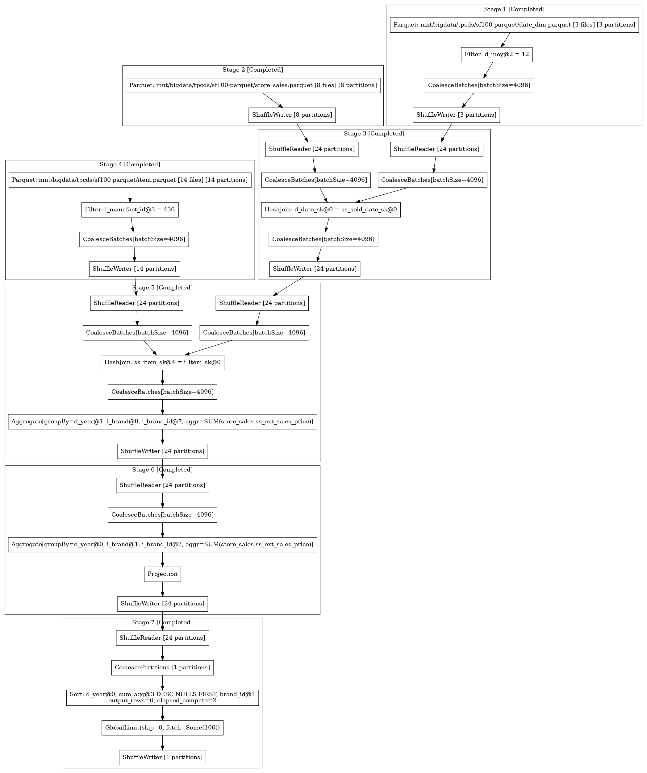
To download a query plan in dot format from the scheduler, submit a request to the following API endpoint
http://localhost:50050/api/job/{job_id}/dot
The resulting file can be converted into an image using graphviz:
dot -Tpng query.dot > query.png
Here is an example query plan: